K-NN Image Classification Using Scikit-Learn
Published on by John Kosmetos
Overview
In this tutorial I'm going to go over the basics of image classification using a very popular ML algorithm, namely: K-Nearest Neighbour. I'm going to use Scikit-Learn's classification implementation, and train it on MNIST (Handwritten digits) data downloaded from OpenML, after which we'll check its accuracy and spot-check a few classifications to see if it works.
What Even Is K-NN?!
Good question! K-NN is a type of supervised machine learning algorithm that assumes "sameness" based on proximity of data points in a given feature space, which is just a fancy way of saying that it groups data that sits close together.
It is considered a lazy algorithm, in that it doesn't produce a model per se, but instead stores data / distances in memory, and predicts on the fly, so it just throws everything into a dict or array and keeps growing it (good for small datasets, bad for biggens).
It is usually one of the first models you learn when stepping into the world of data science due to it's simplicity. There are a few different "flavours" of Nearest Neighbour algorithm, but for the purposes of this post, I'm going to focus on the most straightforward of the bunch, plain old Standard K-NN, but another widely used variant is Weighted K-NN, which I'll cover separately.
How It Works
In its simplest form a K-NN model only needs two parameters to function, the k value, and the distance metric. The k value represents the number of neighbours to take into account when a new data point is added to the feature space, and the distance metric stipulates which measure should be used to calculate the distance between data points. Euclidean distance is used the vast majority of the time, but Manhattan and Minkowski distance are also widely used.
For Classification
In a classification task, the training data will consist of features accompanied by labels. K-NN can handle both singular and multi-label classifications, but for the sake of simplicity, we'll only focus on singularly labelled data.
Let's say that k=3, and the distance metric is set to euclidean distance; when a new data point is added to the feature space, the algorithm first calculates the euclidean distance from the new unseen point to every other point present in the training data, after which it grabs the k closest ones, which in this case is 3, checks their labels, assigns the most prevalent one to the new point, and voila, it is done!
For Regression
With regression tasks, instead of assigning a label, training feature values are used to calculate the median or mean (depending on the task at hand) value to "predict" the outcome of an unseen data point. So as above, assuming a simple implementation, the values of the 3 closest neighbours are merely averaged and returned, easy peasy!
Common Use-Cases
Nearest neighbour algorithms are particularly useful for image recognition, handwriting recognition, spam detection and even financial forecasts (regression). In this post I'm going to use image recognition as an example, specifically handwritten digit recognition.
Example
Time to get our hands dirty, let's jump straight into an example.
Requirements
Before we start, make sure you have your python environment set up and ready to go with the following libraries:
Utility Functions & Imports
To make life a little easier, here are a few utility functions to help with plotting and displaying data, along with all the necessary imports.
import matplotlib.pyplot as plt
from sklearn.neighbors import KNeighborsClassifier
from sklearn.model_selection import train_test_split
from sklearn.datasets import fetch_openml
from sklearn.metrics import confusion_matrix, ConfusionMatrixDisplay

def plot_digits(digits, predictions, classifier_name=""):

    # Generate subplots
    _, axes = plt.subplots(nrows=1, ncols=8, figsize=(15, 2))

    for ax, image, prediction in zip(axes, digits, predictions):

        # Turn off the axis display
        ax.set_axis_off()

        # Reconstitute the image
        image = image.reshape(28, 28)

        # Display image
        ax.imshow(image, cmap=plt.cm.gray_r, interpolation="nearest")

        # Set the title
        ax.set_title(f"Prediction: {prediction}")

    plt.suptitle(f'First 8 {classifier_name} Predictions', fontsize=14)

    plt.tight_layout(rect=[0, 0.03, 1, 0.95]) # Adjust layout to prevent title overlap

    # Show the plot
    plt.show()

def generate_confusion_matrix(true_labels, predicted_labels, labels):

    # calculate the confusion matrix
    cm = confusion_matrix(true_labels, predicted_labels, labels=labels)
    cm_display = ConfusionMatrixDisplay(confusion_matrix=cm, display_labels=labels)
    cm_display.plot()

    # Set the title
    plt.title('Confusion Matrix')

    # Show the plot
    plt.show()
Data Pre-processing
We're going to download our dataset from OpenML and do some basic pre-processing, as follows:
# Load the MNIST dataset from OpenML
mnist = datasets.fetch_openml('mnist_784')

# Get the first 1000 records for now
all_features = mnist.data.to_numpy()[:1000] # The image data
all_labels = mnist.target.astype(int).to_numpy()[:1000] # The corresponding labels, (0-9)
Training & Classification
Before training the classifier, it's a common practice to split your data into training and testing data. This is done to ensure that the model tests against "unseen" instances, and not on data its just been trained on, which would lead to unreliable accuracy scores.
Scikit-Learn has built-in method to do just that called train_test_split, so let's segment the data into a 80%/20% train/test set as follows.
# Split the dataset into training and testing sets
training_features, testing_features, training_labels, testing_labels = train_test_split(all_features, all_labels, test_size=0.2, random_state=42)
Once the data's been split, we're ready to instantiate our model, and start the fitting (training) process.
# Instantiate KNN classifier
knn_model = KNeighborsClassifier(n_neighbors=3)

# Train (fit) the model
knn_model.fit(training_features, training_labels)
Depending on the amount of data and the beefiness of your machine you're training on, this might take some time, but when its done, the only thing left to do is to test your newly trained KNN model on some unseen data, so let's do it,
# Make predictions
predicted_labels = knn_model.predict(testing_features)

# Spot check a few
plot_digits(testing_features, predicted_labels)
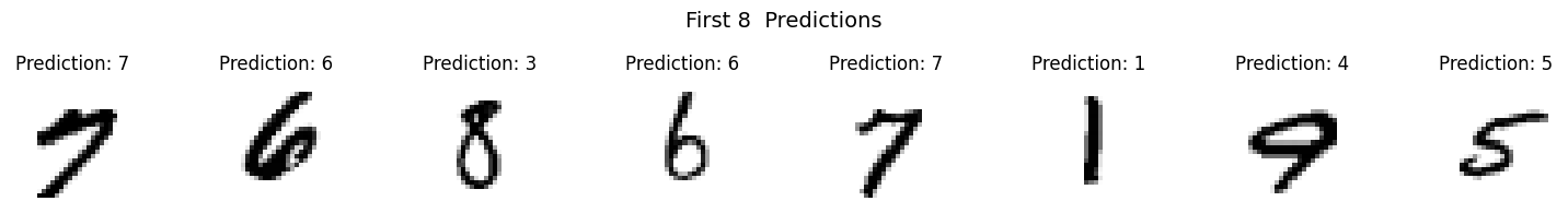
Looks like it correctly classified 75% of the unseen spot-checked digits, and considering we only used 800 training records, that's not bad at all! Some more training, and this model will be humming along nicely.
Evaluation
We're going to use a confusion matrix to check the model's predicted vs true values, to ascertain whether it's any good at generalising to unseen data.
# Generate the confusion matrix using the utility function included above
generate_confusion_matrix(testing_labels, predictions, labels=knn_model.classes_)
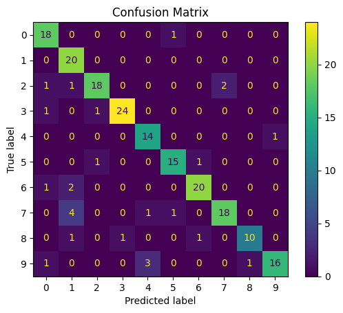
The actual label is denoted via the y-axis, and our model's predicted label via the x-axis. By the looks of it, the majority of the predictions are correct, but let's check one last thing, the overall accuracy.
# Manually calculate accuracy
correct_predictions = 0
for i in range(len(testing_labels)):
    if predicted_labels[i] == testing_labels[i]:
        correct_predictions += 1

# Correct predictions over total number of testing labels
accuracy = correct_predictions / len(testing_labels)

# Print the output
print(f"KNN Accuracy: {accuracy:.2f}")
As shown above, we loop through and compare the predicted and true labels for all test data, then calculate the average. Although Scikit-Learn has built in functionality to calculate this automatically, I wanted to do it manually to show you how easy this is to work with.
When all's said and done, we end up with a 86% accurate model trained on just 800 records, and tested against 200 unseen digits: KNN Accuracy: 0.86.
Accuracy is the simplest of all the classification metrics, but recall and f1-score should be used as well to get a holistic view of your classifier's performance.